

Gem-2 - How it works - Detailed
Click on one of the products to learn more.
The GEM-2 is a hand-held, digital, multi-frequency broadband electromagnetic sensor. It operates in a frequency range of about 30 Hz to 93 kHz, and can transmit an arbitrary waveform containing multiple frequencies. The unit is capable of transmitting and receiving any digitally-synthesized waveform by means of the pulse-width modulation technique.
Depth of exploration for a given earth medium is determined by the operating frequency. Therefore, measuring the earth response at multiple frequencies is equivalent to measuring the earth response from multiple depths. Hence, such data can be used to image a 3-D distribution of subsurface objects. Results from several environmental sites indicate that multi-frequency data from the GEM-2 is far superior to data from single-frequency sensors in characterizing buried, metallic and non-metallic targets.
Introduction
Of many geophysical exploration techniques, the electromagnetic (EM) method provides significant advantages for shallow geophysical exploration.
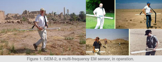
The GEM-2 ‘ski’ is shown in Figure 1. The sensor, weighing about 9 pounds, operates in a frequency band between 30 Hz to about 93 kHz. Its built-in operating software allows a surveyor to cover about one acre per hour at line spacing of five feet. Along a survey line, the data rate is about two per foot, resulting in about 20,000 data points per acre per hour. Such portability, survey speed, and high data density are important requirements for geophysical surveys at environmental sites.
Advantages of a broadband, multi-frequency, EM sensor are obvious. The idea of using multiple frequencies stems from the skin-depth effect, which is inversely proportional to frequency: a low-frequency signal travels far through a conductive earth and, thus, “sees” deep structures, while a high-frequency signal can travel only a short distance and thus, “sees” only shallow structures. Therefore, scanning through a frequency window is related to depth sounding. Figure 2 shows a nomogram from which one may determine the skin depth for a given frequency (Won, 1980)
Using the main software called WinGEM2 in a Windows environment, a PC connected to the GEM-2 can upload the operating parameters to the GEM-2, then download the data after the survey. For more information on WinGEM2, please consult the Operator’s Manual.
Depth sounding by changing the transmitter frequency is called “frequency sounding,” which measures the target response at many frequencies in order to image the subsurface structure. Because the method involves a fixed transmitter-receiver geometry, the sensor can be built into a single piece of hardware, such as GEM-2; as a result, it produces extremely precise, sensitive, and thermally stable measurements. In contrast, depth sounding by changing the separation between the transmitter and receiver is called “geometrical sounding,” which usually requires multiple operators tending separate coils connected by wires and measuring consoles. Maintaining a precise coil separation is difficult and, therefore, some measurements (e.g., in-phase components) are often abandoned. For shallow surveys, the frequency sounding method offers high spatial resolution, survey speed, light logistics, and data precision.
GEM-2 Principle of Operation
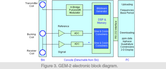
Figure 3 shows the electronic block diagram of the GEM-2. The sensor contains a transmitter coil and a receiver coil separated by about 1.6 meters. Such geometry is called “bistatic” configuration. It also contains a third “bucking coil” that removes (or bucks) the primary field from the receiver coil. All coils are molded into a single board (dubbed “ski”) in a fixed geometry, rendering a light and portable package. Attached to the ski is a removable signal-processing console.
For frequency-domain operation, the program prompts for a set of desired transmitter frequencies. Built-in software converts these frequencies into a digital bit-stream which is used to construct the desired transmitter waveform for a particular survey. This bit-stream controls the H-bridge transmitter driving the transmitter coil to generate a complex waveform that contains all frequencies specified by the operator. The base period of the bit-stream for the GEM-2 is set to 1/30th of a second for areas having a 60-Hz power supply as in the U.S. The period can be set to 1/25th of a second for 50-Hz areas, as in Europe and Japan. Any integral number of the base period may be used for a consecutive transmission in order to enhance the signal-to-noise ratio.
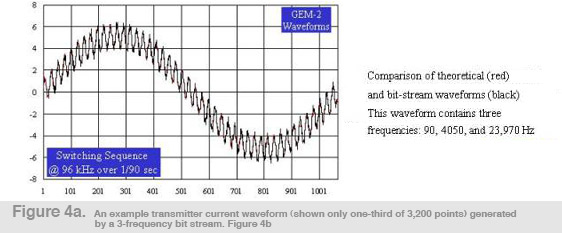
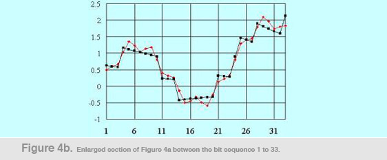
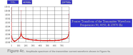
In Figure 4a, we show an example transmitter current waveform, generated by a bit-stream designed to transmit three frequencies, 90Hz, 4,050Hz, and 23,970Hz. The graph shows the current waveform for the bit sequence from 1 to 1,067, the first third of the base period, 1/30th of a second. Figure 4b depicts the waveform details for the first 33 bits, showing the current flow in the transmitter coil. Each bit in this case lasts for 1/192,000 seconds. Figure 4c shows the amplitude spectrum of the transmitter current waveform of Figure 4a. The maximum current (peak to peak) for the present transmitter is close to 10 amperes, corresponding to a dipole moment of about 3 A-m2. Note that the transmitter current decreases logarithmically with frequency.
The GEM-2 has two recording channels: one from the bucking coil (called the reference channel) and the other from the bucked receiver coil (called the signal channel). Both channels are digitized at a rate of 192,000 Hz and 24-bit resolution. This produces a 6,400-long time-series per channel during a base period. In order to extract the inphase and quadrature components, we then convolve (i.e., multiply and add) the time-series with a set of sine series (for inphase) and cosine series (for quadrature) for each transmitted frequency. This convolution renders an extremely narrow-band, match-filter-type, signal detection technique. A single computer in a DSP chip coordinates all controls and computations for both transmitter and receiver circuits.
GEM-2 may also be used to measure the background environmental noise spectrum. This is obtained from the signal-channel time-series at a typical location within a specified survey area, then computing its entire Fourier spectrum at an interval of the base frequency (30 Hz). Using the environmental noise spectrum, the operator can safely avoid locally-noisy frequency bands.
Basic Measurement Unit
These ppm values are the raw data logged by the GEM-2. It is obvious that the ppm unit defined above is sensor-specific and has little physical meaning. All parameters required for the ppm computation, such as the sensor output in free-space (simulated by hanging GEM-2 from the top of a tall tree), amplifier characteristics of the two receiving channels, and the coil geometry, are stored in GEM-2 for real-time use.
In most shallow geophysical surveys, the ppm data generated by GEM-2, often plotted on a contour map for each frequency, are sufficient to locate buried objects without going through elaborate processing or interpretation. One can also estimate the target depth from the data obtained at multiple frequencies.
This mode of operation, called a “bump finder” survey, is appropriate and productive where there are numerous shallow, small, nondescript targets and the survey objective is to find as many targets as possible. The goal is not to determine a detailed geometry for each object, given typical time constraints and the large quantities of objects to be detected. In such a survey, the in-phase and quadrature ppm data are sufficient to indicate the location, size, and depth of a “bump” without converting the data into any other more physically meaningful quantities
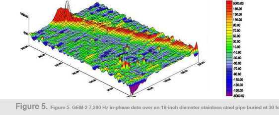
Figure 5 is shown as an example; we look for a buried pipe and our main interest in this case is its location. This figure shows the GEM-2 in-phase response at 7,290 Hz over a known stainless-steel pipe of 18-inch diameter, buried at a depth of approximately 30 feet. A magnetic survey failed to detect the pipe, presumably because it is made of stainless steel, a non-ferrous metal. In this example, the plot showing the ppm response is sufficient to locate the pipe. The survey over this pipe included seven frequencies, and the response was highly dependent on frequency. For example, the pipe was not recognizable at around 2 kHz or 12 kHz.


Conversion to Apparent Conductivity
Since the in-phase and quadrature ppm data contain all information on the measurement geometry, they can be the raw input for any inversion software. Traditionally, however, EM data are displayed in “apparent conductivity” by imagining that the earth below the sensor is represented by a homogeneous and isotropic half-space. While the earth is heterogeneous with regard to geologic variations, it can be represented by an equivalent homogeneous half-space that would result in the same observed data.
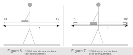
GEM-2 measures the secondary field from the earth (and buried objects therein) at frequencies specified by the operator. When the field is normalized against the primary field at the receiver coil, it is called the mutual coupling ratio (Q), which, for horizontal coplanar mode (or vertical dipole mode), can be written in equation 2 as:
The sensor geometry with respect to the earth is shown in Figure 6. The kernel function R corresponding to a uniform half-space is given in equation 3:
- where
- Hs: secondary field at receiver coil,
- Hr: primary field at receiver coil,
- r: coil separation,
- h: sensor height,
- J0: zeroth-order Bessel function,
- f: transmitter frequency (Hz),
- µ: magnetic susceptibility, and
- s: earth conductivity.
We note that the ppm unit defined by Eq. (1) is the same as Q multiplied by one million. GEM-2 can be configured to a vertical coplanar mode (or horizontal dipole mode) by simply turning it 90 degrees about the ski axis (Figure 7). The mutual coupling ratio for is given in equation 4 as:

where J1 is the first-order Bessel function. The integrals in Eqs. (2) and (4), known as the Hankel transform integrals, can be computed by the linear digital filter method with known filter coefficients for a fast digital convolution (Kozulin, 1963; Frischknecht, 1967). We notice from the above equations that conductivity and frequency appear as a single product. For multifrequency data, therefore, Eqs. (2) and (4) provide the relationship between the ppm unit and the conductivity-frequency product.
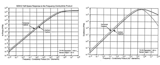
Figures 8 and 9 bleow illustrate the computed in-phase and quadrature responses over half-space for the GEM-2 horizontal and vertical coplanar coils. We assume for this example the sensor height at 1 meter, typically waist level for a surveyor. In essence, the observed ppm value (y-axis) determines the conductivity-frequency product (x-axis), which is then divided by the transmitter frequency to obtain the half-space conductivity.
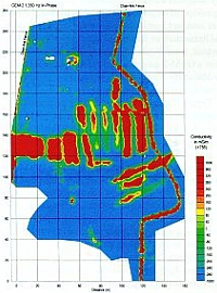
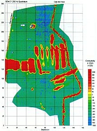
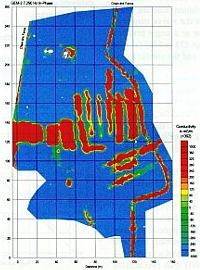
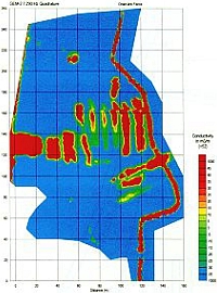
As an example, Figures 10a through 10d show the GEM-2 apparent conductivity data, in units of millisiemen/m (mS/m), over a 6-acre trench complex in the southeastern U.S. Materials, including radioactive waste, were “systematically” buried in many parallel trenches.
1,350 Hz in-phase
10a
1,350 Hz quad
10b
7,290 Hz in-phase
10c
7,290 Hz quad
10d
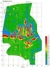
Mag, total
10e
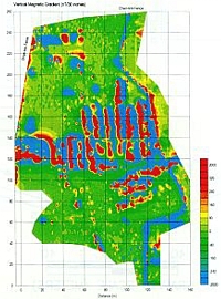
Mag, total vertical
10f
For comparison, Figure 10e shows, for the same area, the total-field, magnetic anomaly map, while Figure 10f shows the total-field, vertical magnetic gradient. For the magnetic data, we employed a cesium-vapor magnetometer (Geometrics G-858G) with two sensing heads vertically separated by 30 inches.
Magnetic anomalies are inherently dipolar in nature and, thus, a target is commonly located at the slope, rather than the peak, of an anomaly. This problem of target location renders the magnetic anomaly hard to interpret, particularly for a target made of many individual items such as drums and cans buried in these trenches. In contrast, it can be shown theoretically by forward modeling that a GEM-2 anomaly is almost monopolar centered directly above the target and, consequently, is easier to interpret than dipolar magnetic anomalies.
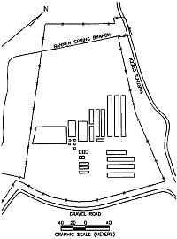
Figure 10g is from an old facility engineering drawing that supposedly shows the trench locations. We do not know whether this old drawing was intended to show the design plan before, or the “as-built” map after, the trench construction. Regardless, it is obvious that the trenches implied by the GEM-2 data are significantly dissimilar from those indicated by the old map. In the end, we concluded that the GEM-2 data best depicts the current trench distribution; therefore, the geometrical boundaries determined from the GEM-2 data were used to compute the waste volume within the trenches. Each map, depicting the apparent conductivity derived from the in-phase and quadrature data at 1,350 Hz and 7,290 Hz, shows a slightly different picture of the trenches. Presumably, the low-frequency data indicate the deep trench structures, while the high-frequency data indicates the shallow trench structures. For plotting convenience, each conductivity map, Figures 10a through 10d, has an average conductivity value (noted on the top of the color scale bar) removed in order to balance the color distribution.
Conclusions
Of the many geophysical sensor technologies, the EM method provides significant advantages for shallow environmental characterization. Unlike seismic or ground-penetrating radar methods that involve heavy logistics and labor-intensive field work, GEM-2 requires only a single operator, does not touch the earth (thus, is less intrusive), and can operate at stand-off distance. An instrument like GEM-2 is ideal for many environmental and geotechnical applications including mapping underground storage tanks, landfill and trench boundaries, certain contaminant plumes, and buried ordnance. In addition, GEM-2 has applications for finding shallow ore bodies for the mineral exploration industry.
With the advent of digital, multifrequency data, we have opened a new dimension in data quality and quantity for imaging and characterizing buried subsurface features. GEM-2 is only the beginning of a new generation of many broadband EM sensors.
References
Frischknecht, F.C., 1967, Field about an oscillating magnetic dipole over a two-layer earth and application to ground and airborne electromagnetic surveys, Quart. Colorado School of Mines, v. 62, no. 1, pp. 1-370.
Kozulin, Y.N., 1963, A reflection method for computing the electromagnetic field above horizontal lamellar structures, Izvestiya, Academy of Sciences, USSR, Geophysics Series (English Edition), no. 2, pp. 267-273.
I.J. Won, 1980, A wideband electromagnetic exploration method – Some theoretical and experimental results, Geophysics, Vol. 45, pp. 928-940.
I.J. Won, 1983, A sweep-frequency electromagnetic exploration method, Chapter 2, in Development of Geophysical Exploration Methods-4, Editor; A. A. Fitch, Elsevier Applied Science Publishers, Ltd., London, pp. 39-64.