
Gem-2 - How it works
Click on one of the products to learn more.
The GEM-2 ‘ski’ is a hand-held, digital, multi-frequency broadband electromagnetic sensor. It operates in a frequency range of 30 Hz to 93 kHz, and can transmit an arbitrary waveform containing multiple frequencies. The unit is capable of transmitting and receiving any digitally-synthesized waveform by means of the pulse-width modulation technique. For a complete description of the sensor, read the Principle of Operation in “The GEM-2 – How it works – Detailed”.
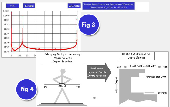
Figure 1. A three-frequency transmitter waveform.
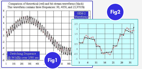
Figure 2. First 33 points of Figure 1.
A frequently-asked question is the “Depth of Investigation.” This is a very complex question because the answer depends on many factors, particularly on ground conductivity and ambient electromagnetic noise. Based on many analyses and field data, we estimate the GEM-2 should be able to see about 20-30m in resistive areas (>1000ohm-m) and about 10-20m in conductive areas (<100ohm-m). This figure assumes an ambient noise level of 5ppm. The noise level is generally high in urban areas and low in rural areas. For typical applications, we do not recommend the GEM-2 for depths deeper than 30m. For more discussion on this subject, consult the Skin depth nomogram in “The GEM-2 – How it works – Detailed”.
The GEM-2 ski contains three coils: transmitter, bucking, and receiver coils. For frequency-domain operation, the GEM-2 prompts for a set of desired transmitter frequencies. Built-in software converts this into a digital “bit-stream,” which is used to construct the desired transmitter waveform (Figs 1 and 2). This bit-stream represents the instruction on how to generate a complex waveform that contains all frequencies specified by the operator.
Figure 3. The base period of the bit-stream for the GEM-2 is set to 1/30th of a second for areas having a 60-Hz power. The TX switches at 192 kHz and, therefore, the bit-stream contains 6,400 steps within the period. Through a Fourier transform of the transmitter current waveform above, we obtain a power spectrum of the primary field, which shows each transmitted frequency.
Figure 4. With multiple frequencies, one can determine layered conductivity structure of the earth, conceptually shown below. This is called “frequency sounding” method. For further discussion, read and article entitled, “Apparent Conductivity (or Resistivity) Revisited” by I.J. Won.